Lecture 15

Simple Harmonic Motion

The simple harmonic motion is very important.  Recall that a particle around any stable equilibrium experiences a restoring force, and thus stays around that stable equilibrium point.  In this lecture, we will see that the resulting motion is a simple harmonic motion, as long as the deviation from the stable equilibrium point is small and assuming that there is no other force (e.g. friction) involved.

Let us be a bit more mathematical.  Consider a stable equilibrium point at a certain value of .  In general, we can take that certain value of  to be zero, simply by shifting the  coordinate system, and so let us do that.  So we are now considering a stable equilibrium point at .  Then, the potential function  must satisfy  and , the first since  is the equilibrium point, and the second since  is the stable equilibrium point, i.e.  is a local minimum at .  Recall from calculus that  .  For small , we can ignore the higher order terms.  Also, noting that  and , and defining , we get

	1. 2. 3. 4. 5. 6. 7. 8. 9. 10. 11. 12. 13. 14. 15. (15.1)
	(15.2)

So, around any stable equilibrium, Hooke's law applies!  The above potential  is called a simple harmonic potential well.  In this lecture, we will consider situations in which the Hooke's law force for  is the only force (however, see comments at the end of this LN), then .  Namely, we have , an equation of motion for us to solve.  It is customary to define

(15.3)

then, the equation of motion becomes 

(15.4)

What is the solution for this?  The general solution is

(15.5)

Some points to note about this solution.

1) How do we know that Eq. (15.5) is the general solution of Eq. (15.4)?  Strictly speaking, it is from the theory of differential equations in mathematics.  [There are many other ways to write down this solution, the most elegant way is perhaps using the complex numbers as in .]  Here is a bit of justification.  Notice that the LHS of Eq. (15.4) is the 2nd derivative of  with respect to .  This means that one expects two “integration constants” to appear in the solution.  Indeed, we have two symbols  and , which did not exist in the original equation (15.4).  This is the correct behavior, and indeed  and  are just (integration) constants.  Next, the 2nd derivative of (15.5) does give , satisfying (15.4).  Let us see this step by step.    [, and the chain rule used here] .   Taking the derivative one more time,   [, and the chain rule used here]  !

2) A few simple problems in classical mechanics are exactly solvable.  We have seen two examples already – the constant acceleration problem (“projectile motion”) and the constant centripetal acceleration problem (“uniform circular motion”).  The simple harmonic motion is our third example.

3)  is the amplitude.  It is taken to be a positive number, by convention.

4)  is the phase constant.  The entire argument of the cosine function, , is called the phase.

5)  is the angular frequency, with the SI unit of Hz (hertz) = 1/sec.  Since  is dimensionless (any argument of sine or cosine is dimensionless, since the angle is a dimensionless quantity), the SI unit of  should be 1/sec.  It is instructive to also check this using Eq. (15.3).  Note that the SI unit of the spring constant  is N/m = .  Thus the SI unit of  is .  Thus, it follows that the SI unit of  is 1/sec.

6)  is independent of  and .

Frequency and period

For any periodic motion, not just for the simple harmonic motion, the following relation applies to the angular frequency (; omega not w), the frequency (; nu not v), and the period (),

(15.6)

Both  and  are widely used.  Using symbol  or explicitly saying “angular frequency” usually removes the ambiguity of which frequency is being discussed.  Another commonly used symbol in place of  is f.

The period () is defined as the time interval to complete one cycle of the motion.  The one cycle corresponds to the change of ange by  for the cosine function.  Above,  is shown with   and a general value.

Meaning of the simple harmonic motion

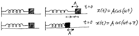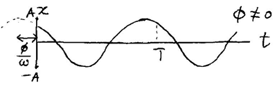
The meaning of the simple harmonic motion seems simple enough.  Consider a frictionless surface on which a mass lies.  The mass is connected to a spring.   Imagine that you pull a mass connected to a spring by a certain distance , and then just release it.  Then, the mass will be pulled by the spring and will decrease all the way to  and then come back to  and so on and so forth.  According to Eq. (15.5), the motion of the mass from then on is completely described by the equation .  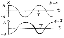The reason why  (modulo 2) is because only then  will have a maximum at .  Suppose that you instead push the spring by the distance , and then release it.  In this case, .

Now, notice that the relation  is exactly like that of the uniform circular motion.  What does the simple harmonic motion have to do with the uniform circular motion?  A lot!  If you allow the circular motion to be a virtual one.  For the mass on spring problem, imagine a virtual world where the same mass is connected to the same spring (or just a string), but this time making a uniform circular motion with the radius , angular velocity  (> 0 for a CCW motion, which is what we consider here), and the initial angle  (measured from the axis).  The following table applies.  UCM = uniform circular motion, SHM = simple harmonic motion.

	UCM in the virtual plane	SHM in the real space
Dimensionality	Two dimensional motion	One dimensional motion
Coordinates		(=  of the virtual plane)
	Initial angle; initial phase	Initial phase; phase constant
	Angle at time	Phase at time
	Angular velocity	Angular frequency
	Period	Period
	Radius	Amplitude
Force	Constant; Centripetal force	Varying (  component of the virtual one)
	component of the centripetal force	The actual spring force

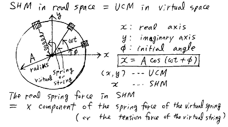What do we learn from this comparison?  That the real world (the SHM) can be thought of as a “mere projection” or a “mere reflection” of the virtual world (the UCM).  [Mathematically, this virtual world is none other than the plane of the complex numbers (“complex plane”) where the  axis is called the imaginary axis.]

One note about the word phase.  The phase of the Moon is determined by the angle of its circular motion around the Earth.  So, it should not surprise you that physicists use words phase and angle interchangeably.

Mechanical energy in a SHM

We already know that the total mechanical energy in a SHM is conserved, since the spring force is a conservative force.  One can check this explicitly.  The kinetic energy is .  In the last step,  has been used.  The potential energy is .  To summarize

(15.7)

Using the well-known trigonometric identity,  (here  is just a dummy symbol; you can replace it with any other symbol), we get

(15.8)

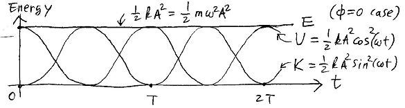Note that  is the maximum displacement, which occurs at turning points where , and  is the maximum speed, which occurs at the bottom of the potential well at .

Other examples of SHM

Around any stable equilibrium point, there is a simple harmonic motion, and so it is easy to come up with other examples of SHM.  [In the following examples, we will be considering real circular motions with small amplitudes as SHMs.  These circular motions are clearly different from the virtual circular motions discussed above.  These real circular motions are non-uniform circular motions and they are restricted to a small part of circle.]

Note that, as in the example of a simple pendulum bob (LN 12), the potential function can be a function of angle, e.g. , instead of a linear coordinate such as .  In that case what is the meaning of ?   It is the torque ().  Recall that the potential energy is defined as work done against a conservative force.  Work in the case of rotational motion is given by .  Thus,  (the minus sign means work done against the force), and so for a rotational motion we get

	(15.9)
	(15.10)

Note the subtle difference in notation here.  We are using  (kappa) not  here.  These equations are the complete rotational analog of Eqs. (15.1) and (15.2), and thus it follows that  will satisfy

(15.11)

It is important not to be confused by the symbols here.   [Keep in mind that any symbol is just a name, and it is what you define it to be.]  Here,  is doing a SHM.  Its phase is , which is the angle in the virtual space, and this phase is distinct from the physical angle, , of the real space.  Note that in this LN we are careful not to call the argument inside the cosine function (; the phase)  since that would amount to using the same symbol again to mean a different thing.  Note also that here  is an angular amplitude.

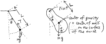Simple pendulum and physical pendulum  The diagram shows a simple pendulum (mass on a massless rod or string) and a physical pendulum, each of total mass .   It is easy to see that the only source of non-zero torque is the gravitational force (the tension force is anti-parallel to the position of the mass and thus gives a zero torque), and the torque is given by  (the  sign means that the direction of  is into the paper, while the positive direction of  is out of the paper).  The equation of motion is then

(15.12)

In general this equation of motion is not solvable, and is different in form from Eq. (15.4).  But, for small  (in radians), , and so we have, for small oscillations of a pendulum (simple or physical),    

(15.13)

Comparing this equation to Eqs. (15.3) and (15.4), we can thus conclude that  will show a SHM, as long as  remains small, with the angular frequency

(physical, or simple, pendulum)

(15.14)

For the simple pendulum,  and so

(simple pendulum)

(15.15)

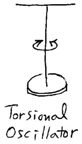Torsional oscillator  If you twist a thin wire, then it has a tendency to go back to its natural state.  In this case, the rotational analog of Hooke’s law, Eq. (15.10), applies.  This torque, , is equal to , where  is the rotational inertia of an object attached to the wire.  Accordingly, the object will go through a SHM, with 

(torsional oscillator)

(15.16)

Damped and driven oscillations

In real life, there is always a source of damping (e.g. friction) and also there can be a source of force that drives the oscillation.  A child on a swing is a good example.

Without friction, the swing motion should be a SHM, driven only by the force of gravity, as in a simple pendulum or a physical pendulum, considered above.  Just like in the examples studied in this lecture note, the frequency of this SHM is determined by the mass, the shape, and the surface gravity.  This frequency is generally called the natural frequency.  Any stable object has a SHM associated with it, and so has a natural frequency.

However, in reality, without pumping the oscillation of a swing dies down (damped oscillation) due to friction.  A child can pump the swing, causing the amplitude increase (driven/forced oscillation).  When a child pumps the swing, she knows instinctively to do this in a regular interval that corresponds exactly to the period of the swing motion itself.  Namely the force/torque applied has the same period as the motion of the swing itself.  When this occurs, the pumping is the most effective.  The condition that the frequency of the driving force/torque is identical with the natural frequency of the oscillating object is called the resonance condition.  Accordingly, a resonant oscillation refers to a driven/forced oscillation where the resonance condition is met.  In general, the effect can be very pleasant (like the sound of a string amplified by the chamber of a violin or a guitar through the resonant oscillation of air in the chamber) or detrimental (like a wine glass shattered by a high pitch voice of an opera singer or, in fact, any curious student).  For design of mechanical objects, such as cars and bridges, the resonant frequency is an important factor to consider – you want to avoid any environmental disturbances/vibrations driving your object with a resonant frequency!

The mathematics of damped and driven oscillations is beyond the scope of physics at this level.  [Read 13.6 and 13.76 of text, for an optional glimpse.]