Lecture 4
Vectors
Definition of vector
A vector
is a mathematical object that is characterized by direction as well as magnitude.
This is not a rigorous definition but it is good enough. Visually, it is an arrow,
pointing from tail to head. Thus, vector quantities are written with an arrow
above them, as in ![]() (force)
or
(force)
or ![]() (velocity).
(velocity).
Vector addition
To add
two vectors, (1) translate one of the two vectors so that its head is on the
tail of the other vector, and (2) draw a new arrow starting from its tail to
the head of the other vector. There are two ways to do this, depending on
which vector you choose to move, and they give the identical result, i.e., the
vector addition is a commutative operation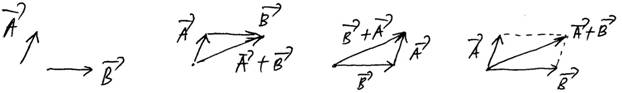 :
: ![]() .
Another way to add two vectors is (1) bring the tails of the two vectors to a
common point, (2) complete a parallelogram starting from the two sides
corresponding to the two vectors (see dashed lines above), and (3) draw an
arrow from the common tail point of (1) to the new vertex of the parallelogram
created in (2).
.
Another way to add two vectors is (1) bring the tails of the two vectors to a
common point, (2) complete a parallelogram starting from the two sides
corresponding to the two vectors (see dashed lines above), and (3) draw an
arrow from the common tail point of (1) to the new vertex of the parallelogram
created in (2).
 Vector subtraction
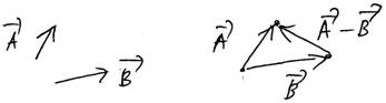
The subtraction
is the inverse operation of addition. Be sure to understand the example diagram
as ![]() .
.
Multiplying a vector by a scalar
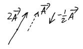 For a
given vector
For a
given vector ![]() ,
,
![]() ,
where
,
where ![]() is
a number (i.e. a scalar), corresponds to scaling that vector. If
is
a number (i.e. a scalar), corresponds to scaling that vector. If ![]() is a positive number, then it
means stretching or contracting the size of the vector. If
is a positive number, then it
means stretching or contracting the size of the vector. If ![]() is a negative number, then it
means changing the direction of the vector and then stretching or contracting
it.
is a negative number, then it
means changing the direction of the vector and then stretching or contracting
it.
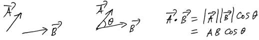
Multiplying two vectors – scalar product
One way to multiply two vectors is to form the so-called the scalar product. The definition is
|
|
|
(4.1) |
where ![]() (B) means the magnitude
of
(B) means the magnitude
of ![]() (
(![]() )
and
)
and ![]() is
the angle between
is
the angle between ![]() and
and ![]() .
.
Thus far, we have defined vector addition and two kinds of multiplications. Any combinations of these operations are commutative and associative, just like for ordinary number addition and multiplication.
 Components
While
the above rules are good for visualizing operations on vectors, they are often
cumbersome for calculations on vectors. For the latter, we need to represent
a vector: that is (1) define a coordinate system, (2) project the vector onto
the axes of the coordinate system, and (3) read the numbers at the projection
points – these numbers are called “components.” A collection of components,
e.g. ![]() for
a 2D vector
for
a 2D vector ![]() ,
is called a representation of
,
is called a representation of ![]() .
.
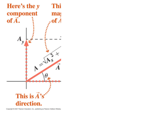
Components as Cartesian coordinates
The most basic coordinate system is the Cartesian coordinate system. For this course, it is sufficient to consider a 2D Cartesian coordinate system. This is illustrated in the figure above. The following relations should be understood thoroughly (not memorized!) in order to go between “the magnitude, direction description of a vector” and “the component representation of a vector.”
|
|
|
(4.2) |
|
|
|
(4.3) |
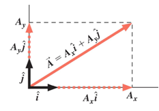 Unit vectors
A unit vector for a given axis of
the coordinate system is the unit-length vector that points to the positive
direction of that axis. Notations ![]() are
used to denote unit vectors for
are
used to denote unit vectors for ![]() axes
respectively. So are notations
axes
respectively. So are notations ![]() . From the above definition of
components, it follows that (for 2D, with a straightforward generalization to
any dimensions):
. From the above definition of
components, it follows that (for 2D, with a straightforward generalization to
any dimensions):
|
|
|
(4.4) |
|
|
|
(4.5) |
Position, displacement, velocity, and acceleration vectors
Any
position in space is a vector, in the sense that, once the origin of space is
given, one can draw an arrow from the origin to the position. A position
vector is usually denoted as ![]() .
.
Displacement is another vector
quantity. It is defined as the difference between two position vectors: ![]() .
.
Here we give the definition of velocity and acceleration vectors in any general dimensions. [That is, the definitions (2.1) through (2.6) are merely special 1D cases of these.]
|
Average velocity |
|
(4.6) |
|
Velocity |
|
(4.7) |
|
Average speed |
Time average of the
instantaneous speed |
(4.8) |
|
Speed |
|
(4.9) |
|
Average acceleration |
|
(4.10) |
|
Acceleration |
|
(4.11) |
Note
(again) that the three vector quantities ![]() are
the most fundamental quantities here, from which all other quantities can be
derived.
are
the most fundamental quantities here, from which all other quantities can be
derived.
Vector calculations in terms of components (or “why components are cool”)
For two
dimensional vectors ![]() and
and
![]() ,
the following holds.
,
the following holds.
|
|
|
(4.12) |
|
|
|
(4.13) |
|
|
|
(4.14) |
|
|
|
(4.15) |
|
|
|
(4.16) |
|
|
|
(4.17) |
Note that all these rules, except the last one, can be called “component-wise” rules. I.e., identity, addition, subtraction, scaling, and differentiation operations of vectors can be performed component-wise. This is the basis of “divide and conquer rule” that we will use in the next lecture. Namely, a 2D problem can be divided into 2 sets of easy 1D problems, using the component representation.
What more about vectors?
This
lecture summarized all things about vectors, to the extent as necessary in this
course, except one thing – the vector product, ![]() .
We will cover that when we learn about torque and angular momentum, later in
this course. The vector product is an odd operation – it is not commutative,
but rather anti-commutative:
.
We will cover that when we learn about torque and angular momentum, later in
this course. The vector product is an odd operation – it is not commutative,
but rather anti-commutative: ![]() .
In contrast, the scalar product is a commutative operation, as already mentioned
above:
.
In contrast, the scalar product is a commutative operation, as already mentioned
above: ![]() .
.