Lecture 2

Dimension and 1D Kinematics

Dimension

The dimension can be considered as an abstraction of the unit, and is defined as follows.  If the SI unit of a physical quantity Q is , then the dimension of Q is defined as  (L=length, M=mass, T=time).

Note:

(1) The dimension of a physical quantity is unique, but the unit is not.  For example, a velocity can be expressed as 40 mph or 20 m/s, but its dimension is always .

(2) If A = B, then the dimension of A = the dimension of B.  Put another way, if two quantities have different dimensions, they cannot be equal (and thus, they cannot be compared either).

Example 1:   The dimension of the area is  (the SI unit of the area is ; or remember that we measure areas in “square feet”) and the dimension of the volume is  (the SI unit of area is ; or remember that we measure volume in “qubic feet”).

What is the dimension good for?

If you get in the habit of checking the dimension of your answer, that is a habit that can go a long way to make you a good student and a good scientist.  I believe that all scientists have this habit.  The dimension is also the basis of the so-called “dimensional analysis,” which is a very useful technique.  Both points are illustrated by the following simple example.

Example 2:  Given the radius of  m and the mass  kg (for more exact numbers, see the inside cover of the textbook) of the Earth, what is the average density of the Earth?  Since the density = mass / volume, we need to express volume, , in terms of given quantities,  and .  Scenario 1.  You are a math wizard, and you use your multi-dimensional integral calculus skill to derive .  Alas, dimension-wise, this equation does not make sense, since it implies  (cf. the note point (2) above).  Realizing this, you check your calculation and, sure enough, find that you dropped a power of , and correct your expression to , to proceed to the correct answer: density =  (this answer is not terribly accurate, since  and  were given with only one significant figure).  Scenario 2.  Suppose this was a multiple-choice question for your MCAT/GRE/GMAT exam with the following choice of answers:

You are not given the formula , which you don’t remember and don’t have time to figure out.  What to do?  Do not panic, as the dimensional analysis can come to the rescue!  Note that the dimension of the volume is , and so it must be that  (Why?  The dimension of  is , and the dimension of  is .  So the only combination of  and  to give the dimension  is .)  Thus, , i.e. density equals  up to a numerical factor.  You then make an educated guess that this numerical factor is on the order of 1:  i.e. it could be, say, 0.7 or 5, but it just cannot be, say, 300 or 0.05.  Thus, you are pretty sure that the density .  So, you can choose with confidence that (c) is the correct answer.  Your answer is about 5 times too large, which is not surprising at all for a dimensional analysis.  While this example is very simple, the insight given by the dimensional analysis is extremely valuable for many difficult real life problems.

Order of magnitude estimate

As a rule, an order of magnitude (“ballpark”) estimate of an unknown physical quantity of interest is very valuable, since it is much more quickly obtained than a numerically precise answer.  For a solvable problem, a ballpark estimate should be compared with the precise answer.  If they do not agree within the order of magnitude, then it probably means that there were some mistakes made in the (presumably) lengthy process of obtaining the precise answer.  For an unsolved problem, an order of magnitude estimate is the only answer!  [The order of magnitude estimate is closely related to the dimensional analysis described above.]

Example 3: [Wolfson 1.4] How many cells are in a brain?  Circumference ~ 2.5 “span.”  2r = 2.5 “span”.  2r ~ 9 inches ~  20 cm.  Subtract ~ 5 cm for skull bones.  2r ~ 15 cm.  Cube it ~ 3E3  = 3E-3  to get the volume of a brain.  How about the size of a cell?  Red blood cell has diameter ~ 10 m =  m.  So a cell volume ~ .  So, taking the ratio = brain-vol/cell-vol, we get ~ 3E12 cells.  Not too bad!

1D Kinematics

Kinematics

Kinematics means study of motion without specifying the cause of motion.  As opposed to dynamics.   1D = one dimension(al).  2D = two dimensional/dimensions…

Velocity and speed – a simple introduction

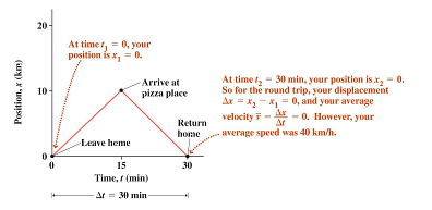
The figure shows a simple sequence of motion, which are summarized in the table below.  In the table note some standard notations: the subscript  meaning “initial” as in , the subscript  meaning “final” as in , the  (Delta – another Greek letter) symbol meaning “the change of” as in  and .

					(min)	(km)
	(min)	(min)	(km)	(km)			= distance	(km/h)	(km/h)
1^st leg	0	15	0	10	15	10	10	40	40
2^nd leg	15	30	10	0	15	-10	10	-40	40
Round trip	0	30	0	0	30	0	20	0	40

Here, the last two columns represent two ways of measuring how fast the trip was.  Let us define some terms here.  We define  as the displacement (change in position),  as the average velocity.  Note that the displacement is a signed number, depending on the sense of direction, and so is the average velocity.  The position, the displacement, and the average velocity each have both the magnitude and the direction – they are vector quantities.  In contrast, quantities with no sense of direction are called scalar quantities.  Here, the distance () and /t (the average speed) are scalar quantities.

Position, velocity and acceleration

In the above example, long time intervals (15 or 30 minutes) were considered.  When the time interval of consideration becomes very very small (“zero within the error” in the physics sense; “infinitesimal” in the mathematical sense), we then talk about “instantaneous” quantities.   So, we come to very important definitions.

Average velocity		1. 2. (2.1)
Instantaneous velocity		(2.2)
Average speed	Time average of the instantaneous speed	(2.3)
Instantaneous speed	The magnitude of the instantaneous velocity	(2.4)
Average acceleration		(2.5)
Instantaneous acceleration		(2.6)

Note:

(1) The position (), the instantaneous velocity () and the instantaneous acceleration () are the most fundamental quantities here.  Incidentally, all of these are vector quantities.

(2) Nearly always the adjective “instantaneous” for  and  can be omitted, since the instantaneous nature is obvious from context.

(3) From the above definition,  is the time-derivative of , and  is the time-derivative of .  Thus,  gives the tangential slope of the graph , and  gives the tangential slope of the graph .  You should carefully study figures 2.4, 2.5, and 2.7 of Wolfson and understand them thoroughly, from this point of view.