Lecture 1

Units and significant figures

What will we learn in this course?

[Please read the syllabus first.] In this course, we will learn very deep principles of physics – Newton’s laws and conservation principles. You will also learn how to do lots of problems, but please try to appreciate the underlying big principles beyond just the “how to” for each problem. That way, you will get closer to the way physicists and scientists think in general, and also you will score better grades.

Unit system

We will mostly use the so-called “SI” unit system (le Système international d'unités). Its old name is the MKS unit system. M is for meter (m), K for kilogram (kg), and S for second (s). These three units for length, mass, and time form the sufficient basis of units for our course, and so they are called “base units.” In general, you will need four more base units (mole for amount, candela for luminosity, ampere for electric current, and Kelvin for temperature), but we don’t need them in this course (6A). The importance of base units is that the unit of any arbitrary physical quantity can be expressed as a product of powers of base units. For example, (as we will learn soon) the SI unit of speed or velocity is m/s = m, and the SI unit of energy is . These units are examples of “derived units,” as opposed to base units. Some derived units have special names: Hz (hertz) = 1/s, J (joules) = .

Unit conversion

There are quite a few unit systems in use, and thus unit conversions are necessary. For example, here is a table for converting some everyday units (or “English units”) such as pounds (lbs), yard (yd), feet (ft), inches (in), and miles to and from appropriate SI units.

SI unit (w prefix)	E unit	E unit, roughly	Comments
1 m	3.28 ft, 1.09 yd, 39.4 in	~ 3 ft, ~ 1 yd	1 yd = 3 ft, 1 ft = 12 in
2.54 cm	1 in
1 km	0.621 miles	~ 0.6 miles	80 km 50 miles
1 m/s	2.24 mph	~ 2 mph
1 kg	2.20 lbs	~ 2 lbs
1 rad	57.3 ^o		rad = 180 ^o

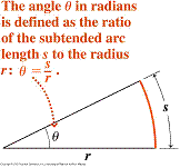The last one deserves more comments. The unit of angle in the SI system is radian. The angle in radians is defined as shown in this figure. So, it follows that radians = 360 degrees, since the circumference of a circle is . You will have to remember this if you didn’t know it already.

Also, note that kg = 1000 g (=grams), cm = 0.01 m and km = 1000 m. Here, k (= kilo) and c (= centi) are examples of unit prefixes (see below).

You should be able to convert units freely in this course. Unit conversion follows the general rules of multiplication and division.

Example 1. 1 m = 3.28 ft. How many yards is 1 meter, given that 1 yd = 3 ft? Answer: 1 yd = 3 ft means that 1 ft = yd. And so,

Example 2. Given that 1 km = 0.621 miles, how many mph (= miles per hour = miles/h) is 1 m/s? Answer: Note that 1000 m = 1 km, which means m = km/1000. Also note that 3600 s = 1 h, which means 1/s = 3600/h. Thus, we get . If you like, you can use clever representations of 1, as follows. 1 km = 0.621 miles means 1000 m = 0.621 miles, which means 1 = 0.000621 miles/m. Also, 3600 s = 1 h means 3600 s/h = 1. Inserting these two clever choices of 1, we get . Note that the symbol “m” appears twice, once in the numerator and once in the denominator, canceling each other out. The same goes for the symbol “s.” Indeed, these canceling-outs were the purpose of the clever choices of 1. This way, we also get 1 m/s = 2.24 mph.

Unit prefixes

We already encountered kilo and centi. The following table summarizes often used prefixes in this course (see textbook for more). For example, 1 nm = m, and 1 MHz = Hz = .

Symbol	G	M	k	c	m		n
Prefix	giga	mega	kilo	centi	milli	micro	nano
Power

Note:

(1) Case matters! Often M (mega) and m (milli) seem to be confused – they are different by 9 orders of magnitude!

(2) Some symbol is Greek! So, micro () is distinct from milli (m). Physicists seem to like Greek symbols, and you will encounter a few of them in different contexts later in this course. Among the “infamous” is , which is omega. You will need to distinguish it from w.

(3) Presumably you’ve heard about giga, mega, and kilo, in relation to computer memory. However, slight differences exist between those computer science definitions and our physics definitions above.

Scientific notation

Any non-zero real number can be written as where (“coefficient”) is a real number satisfying and (“exponent”) is an integer. We define this representation as the “scientific notation.” [Strictly speaking, this is the “normalized” scientific notation, where “normalized” means . I.e., we take the convention to always normalize for the scientific notation.] Often (e.g. in computer codes) or is used to mean . In this course, the notation may sometimes be used to save space.

Number of significant figures/digits

The number of significant figures is defined as the number of digits used for the coefficient in the scientific notation. So, significant digits are those digits that serve the purpose other than representing the order of magnitude (). Also, note that this definition leaves the # of sig-figs of zero (e.g., 0.000) un-defined. One should determine how to represent zero, by investigating the implied error (see below).

Example 3

(# of sig-figs = 1), (# of sig-figs = 4)

(# of sig-figs = 3) , (# of sig-figs = 2)

(# of sig-figs = ambiguous; 1, 2 or 3?), -1001 = -1.001E3 (# of sig-figs = 4)

(# of sig-figs = 1), (# of sig-figs = 2), (# of sig-figs = 3)

Note: Trailing zeros for integers (as in 100) are always ambiguous, while trailing zeros appearing after the decimal point (as in 0.00100) are clearly significant. You will see that many problems in the textbook do use ambiguous expressions such as 100 kg. By convention, we will take this to mean three significant figures. In general, most textbooks seem to automatically imply two or three significant figures when numbers are written ambiguously.

Significant figures and errors

In principle, all scientific numbers should be reported with error estimates, e.g. the Bohr radius (roughly the radius of a hydrogen atom) is m. If all numbers are expressed in this way, there is no need to consider “significant figures” at all. In other words, using the notion of “significant figures” is a poor, but convenient, substitute for explicitly specifying errors. The rough implied error is determined by the rounding rule. For instance, when the surface gravity is written as , it implies that the error is , where ~ means “roughly on the order of.”

Rules of thumb for calculations involving significant figures

These rough rules below are based on the principle that “the least accurate number determines the overall accuracy.” [The virtue of these rules is that they are easy to apply. However, if one were to use explicit errors for all numbers, the error propagation theory must be used instead, leading to a greater complexity. Thus, in essence, significant figures provide a quick and dirty way to deal with errors and their propagation, but you would need to use well-quantified error estimates whenever possible for your professional projects.]

A. Adding (or subtracting) two numbers. (i) Express the two numbers in the scientific notation. (ii) If the two exponents differ, then re-express the number with the smaller exponent by using the larger exponent, which we will call . In this conversion, the coefficient of the re-expressed number will be made smaller than 1 in magnitude, and thus the re-expressed number will no longer be in the scientific notation (i.e. not normalized any more), per our definition above. Anyhow, at this point, we have the two numbers expressed as and . (iii) Now, we can add (or subtract) the two coefficients, and , and let us call the result . Suppose that has digits after the decimal point, and has digits after the decimal point. Then, you should round so that its number of digits after the decimal point is the smaller of and . (iv) Lastly, convert, if necessary, the result to the scientific notation.

B. Multiplying (or dividing) two numbers. If the two numbers have the # of sig-figs, and , then the result should be rounded so that its # of sig-figs is the smaller of and .

C. Complicated functions such as square root, sin, cos, … – the # of sig-figs remains un-changed.

D. For multi-step calculations, keep at least one more sig-figs than that of the final answer, in intermediate steps. This is to prevent the accumulation of rounding errors. [In reality, crunch out numbers with your calculator with high machine precision, and keep the correct number of sig-figs only at the end.]

Unfortunately, the rule A is quite wordy and may seem complicated. This rule should not be forced into memory but should be understood in terms of the underlying principle that “the least accurate number determines the overall accuracy.” Examples should help.

Example 4

(1) 1.3 + 0.001 = 1.3E0 + 1.0E-3 [step (i)] =

1.3E0 + 0.001E0 [step (ii); now ready to add coefficients; 0.001E0 is not normalized] =

1.3E0 [step (iii); 1.3001 rounded to 1.3 since the initial error of the first term dominantly determines the error of the outcome]

This example is so simple that 1.3 + 0.001 = 1.3 would have been clear enough. Let us spell out the meaning of this result. 1.3 + 0.001 = (1.3 ) + (0.001 ). The 2^nd term is clearly insignificant compared to the error of the first term , and so can be safely ignored.

(2) 3.70E2 + 52 =

3.70E2 + 5.2E1 [step (i)] =

3.70E2 + 0.52E2 [step (ii), now ready to add coefficients; 0.52E2 is not normalized] =

(3.70 + 0.52)E2 =

4.22E2 [3.70 and 0.52 have the same digits after the decimal point, and thus the same implied errors, . Steps (iii,iv) are unnecessary.]

(3) 3.7E6 + 5.2E5 [step (i)] =

3.7E6 + 0.52E6 [step (ii)] =

(3.7 + 0.52)E6 =

4.2E6 [step (iii); 4.22 rounded to 4.2 because of 3.7, whose error dominantly determines the error of the outcome]

Let us spell out the last step. The sum 3.7 + 0.52 = (3.7 ) + (0.52 ) = (4.2 ) + (0.02 ). As in (1), the 2^nd term can be ignored to a good approximation. Thus, “the least accurate number determines the overall accuracy.”